Geometry

Overview

A number of terms is going to be introduced in this section (e.g. surface tolerance, surface transparency). These names are specific to SCONE. However, very similar concepts can be found in other codes albeit under different names.

Constructive Solid Geometry

Constructive Solid Geometry (CSG) is a standard way to represent volumes in Monte Carlo codes. Many better references that explain details of how it works are available [Salvat] [Briesmeister], thus only a brief overview will be given here.

In principle, a surface can be represented by an equation \(0 = F(r)\). Thus, for any point in a geometry it is possible to evaluate \(F(r) = c\). Now halfspaces can be defined using the sign of the remainder (\(c\)) of the surface expression. Positive (+ve) halfspace corresponds to \(c > 0\) and is considered an outside of the surface. Similarly, negative (-ve) halfspace is associated with \(c < 0\) and is considered an inside of the surface. Clearly each surface subdivides the entire space into two halfpaces. Ideally there would be no need to consider a case of \(c = 0\), as the probability of finding a randomly placed point exactly at the surface is zero. However, in Monte Carlo transport simulations the movement of the particles is often explicitly resolved, which means that they need to be temporally stopped at the material interface in order to resample their flight distance. As a result, significant care must be taken to ensure a correct behaviour of the geometry implementation in the vicinity of surfaces (small \(c\)).

The binary subdivision of a whole space is rarely sufficient. More practical volumes can be defined with set expressions on the halfspaces. In other words, an almost arbitrary volume can be constructed by unions, intersections and complements (differences). A volume defined in such a way constitutes a cell. It is important to note that a cell does not have to be compact [*] due to the union operation, which can combine disjoint halfspaces. Computationally, it is easiest to deal with cells that are created by intersections only. As a result, such cells are called simple cells. Cells that include other logical operations (unions, complements) will be called just cells or full cells.

Geometry as a Directed Acyclic Graph

With surfaces and cells, it is possible to subdivide the entire space into disjoint regions. In SCONE we call such subdivision a universe. However, it is important to note that in principle this subdivision may be accomplished by other means that the CSG cells introduced in the previous section. Thus, to emphasise this difference, we call the cells that are part of a universe local cells. For some universes they might be CSG cells as well, but they do not have to.

In principle, a single universe is sufficient to perform a simulation. Each local cell could be assigned with a material and that would be complete definition of a problem domain. Such single level representation might be sufficient for a number of problems. However, in the context of a reactor physics, where the problem geometry may be composed of literally tens of thousands individual fuel pins, the single level approach would be cumbersome to a user, error prone and often computationally inefficient. Fortunately, it is possible to take advantage of the repeated nature of the reactor problems via the concept of universe nesting (nested universes or nesting). Instead of filling a local cell in a universe with a material, it is possible to fill it with a nested universe, which is an independent, new subdivision of the entire space. Thus, a cell with a universe filling becomes a portal (the cake is a lie!) into a new universe. Consequently, it is possible that a particle is present in multiple universes simultaneously. Each of these universes is called a level. Thus, if nesting is used, we are dealing with a multi-level geometry. Furthermore, because each cell portal can be associated with a translation and rotation, coordinates on each level may be different.

Universe nesting structure is a significantly different problem from the spatial subdivisions within a universe. It can be represented with a directed acyclic graph (DAG). Each universe can be considered a node in the graph with a transition (edge) associated with each local cell in that universe. Target of a transition is the content of the cell. If the cell is a portal, then the target is another universe node. Otherwise, if the cell is filled with a material, transition points to a node without any transitions of its own. Effectively, it can be though of as a universe filled entirely with a single material. Such material node is called a sink (since it cannot be escaped, it is terminal).

Multi-level geometry must begin with a single starting universe node, which is called a root universe. Now a point can be placed somewhere in this universe. This location is associated with a specific local cell and thus a transition to another node. If the transition leads to another nested universe the process can be repeated until the search terminates in a sink node, which specifies the material at that original point in the geometry. In order to ensure that the search in the graph terminates, the graph needs to be acyclic. If there were cycles (transition paths that lead back to the same universe) there would be a danger that for some points the search would enter an infinite loop.

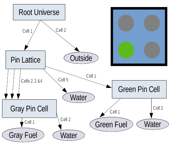
_images/DAG_geom.png — A sample directed acyclic graph representing geometry structure for a simple problem composed of 2x2 lattice of pins.

For illustration, Figure 1 shows a DAG structure of a very simple geometry composed of 2x2 lattice of pins. In SCONE, by definition, root universe is composed of two cells only. One corresponds to the inside of the calculation domain and the other to the outside. Below the root there is a lattice universe composed of five cells in total. Four cells are associated with each pin cell, while the fifth cell defines the composition of the space not occupied by the pin cell lattice. Notice that the size of the windows in root universe is such that only four pin cells are visible. Thus, it is impossible for a particle to be present in the 5th cell in the lattice universe. However, it still needs to be defined because a universe is a decomposition of the entire space into cells. Furthermore, the lattice contains only two different species of fuel pins. Each is associated with a separate nested universe composed of two cells, one defining the fuel pin and the other (stretching to infinity), which defines the surrounding water.

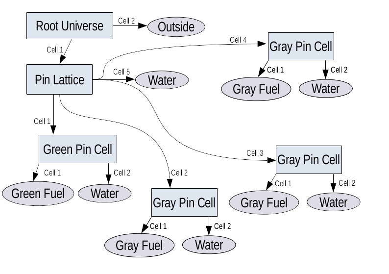
_images/Geom_tree.png — Directed acyclic graph representing the 2x2 lattice after decomposition into a tree by coping instances of the grey pin universe.

The graph structure allows to speak about identity of different cells, even when they are filled with the same material (e.g. water). By enumerating sinks of the geometry graph it is possible to assign a unique ID to each region of space. This capability may be useful for e.g. burn up calculations, in which regions filled originally with the same material can experience different evolution of composition over irradiation time. However, the major problem of the DAG representation of geometry as presented in Figure 1 becomes apparent. It is that the geometry does not distinguish individual grey pin cells. From its point of view it is just a single fuel pin that is present in three different places simultaneously. Clearly the solution would be to copy the grey pin universe to create separate sinks for each instances as shown in Figure 2, which converts the DAG into a tree. This copy could be done “by hand” in an input file, however this is likely to be both error prone and cumbersome to a user.

However, as mentioned earlier, spatial subdivision in a universe and representation of the nesting structure are different problems. It is significant, because the decomposition into a tree needs to be performed only from the point of view of the structure. All of the copied universes share the same description of the spatial subdivision despite bearing different content. In general, description of space requires much more memory then the description of the content. Thus, a considerable amount of memory can be saved if the copied instances of the universe share the description of the spatial subdivision, because in many practical calculations the copied universes may number in thousands.

The problem of assigning unique IDs to material cells can also be looked at from a slightly different perspective by noting that each cell instance corresponds to a unique path in the DAG between source (root universe) and the sink. Thus, the problem of a sink identity can be approached by counting (and enumerating) unique paths in the DAG between root (source) and a particular sink.

Membership at a surface

As it was indicated in previous sections, some care is required when assigning membership of a point to either halfspace of a surface in its vicinity. The main difficulty is caused by the numerical precision of floating point numbers. When particles are moved forward by a calculated distance to a surface, it is desirable that they cross the surface so a new material can be found. However, in most cases the evaluated remainder \(c = F(r)\) of the surface expression will be different from zero after the movement. If an overshoot happened and the \(c\) has changed a sign it is not a problem as the particle has successfully crossed the surface. However, in a case of undershoot the sign of \(c\) will remain the same. This problem can be reduced in frequency by introducing a surface tolerance.

When the surface tolerance is used, the direction of a particle is used to determine its halfspace if the remainder \(c\) of the surface expression is such that \(|c| < surf\_tol\), where \(surf\_tol\) is some small distance representing the surface tolerance. Thus, for example, if \(c\) is within the surface tolerance and a direction of particle is moving it outside the surface, then the particle is placed in the +ve (outside) halfspace. See Figure 3 for further details.

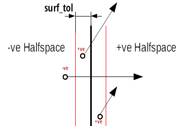
_images/HS_membership.png — Membership in +ve or -ve halfspace for particles close to the surface.

Boundary Conditions

There are two main approaches to the treatment of boundary conditions, which are called explicit and co-ordinate transform. Explicit treatment is more natural and general. In it, an explicit tracking of the system boundary is performed. If a particle is to leak out of the system it is moved to the boundary and the type of boundary condition is checked. If it is vacuum BC, then a particle is removed from the calculation. If it isn’t, any transformation of a particle state can be performed (reflection, albedo reflection or transition in a periodic BCs) after which the distance to a collision is resampled and tracking may proceed as normal.

Co-ordinate transform treatment is more subtle and it is based on the observation that in the majority of problems, reflective and periodic BCs are introduced to convert a finite region into an infinite lattice. If it is the case, it is possible to remove the need for explicit tracking of the system boundary. Instead, a particle is allowed to leave a calculation domain before it is brought back by applying an appropriate number of transformations (reflections by a surface or translations) associated with different faces of the domain boundary. Faces associated with vacuum BCs perform no transformations. Then, if a particle were to escape through one of the vacuum faces, after all transformations are applied, it will be outside the domain and may be considered to have leaked.

Figure 4 illustrates the principle behind co-ordinate transform BCs. Solid colour region is the calculation domain and the semi-transparent is the infinite lattice corresponding to the given boundary conditions. When a particle is moved, it follows the solid line and leaves the calculation domain. Then it is possible to calculate how many transformations are required to bring the particle back to the calculation domain (2 in y-axis, 1 in x-axis). After the transformations are applied, the particle returns to the domain as if it has travelled along the dashed line.

_images/coordBCs.png — Co-ordinate transform boundary conditions. Periodic BCs in vertical direction, reflective BC on right face and vacuum on left face in a-axis. Solid line is a true movement of a particle in geometry, dashed line represents the apparent movement in the domain. Transformations move the particle from the end of the solid line to the end of the dashed line.

Unfortunately co-ordinate transform BCs require that the particle is not stopped when crossing into a new material, thus they can be used only together with Woodcock delta-tracking. Furthermore, the use of the co-ordinate transformations significantly limits the available shapes of the domain boundary and combinations of BCs at different faces. These constraints originate from the requirement that the domain must be translatable into an infinite lattice. For example, a hexagonal boundary with a mix of reflective and periodic boundary distinctions is not allowed.

Distance calculation & Surface Crossing

In order to track particles in the geometry it is necessary to have an ability to calculate the distance to a point along the direction of flight where material composition or unique cell ID changes. This can happen only at the boundaries of local cells in a universe. The main complication in calculating the distance is related to the multi-level structure of the geometry. Since the particle exists in multiple universes at different levels simultaneously, it is necessary to calculate the distance to the next local cell in each of them and take the minimum. The result of this process is both the distance as well as the level at which particle will cross to the next cell.

It is possible that the distance to the next cell will be the same at two different levels. If it happens, it is necessary to take the value on the higher (closer to root) level. When performing this selection it is crucial to account for floating point precision. Floating point numbers \(a\) and \(b\) are considered equal if \(\frac{|a-b|}{b} < \epsilon\), where \(\epsilon\) is some small constant (e.g. \(1.0e^{-10}\)).

Finite precision of the floating point representation causes yet another problem. In a case of an undershoot (where a particle should reach a surface, but is placed slightly before it) a particle may get stuck. For a particle very close to a surface the distance may be so small that if a particle is moved by it, its coordinates will not change (adding FP number to a much larger FP number). Because, this small distance is likely to be chosen as the next transition, particle will not be moved and the same problem will reoccur in the next distance calculation causing and infinite loop.

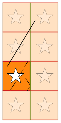
To avoid the infinite loop it is necessary to introduce the surface transparency. Its principle is illustrated in Figure 5 for the bottom particle. If a particle is within \(surface\_tol\) of the surface, the closest crossing (as absolute value of distance along the flight direction) must be ignored for a purpose of distance calculation. It is crucial to remember that the \(surface\_tol\) is defined as a normal distance to the surface. Thus ignoring a crossing distance \(d\) if \(d < surface\_tol\) is insufficient.

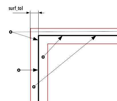
_images/DistCalc.png — Distance that should be returned for particles in different positions close to the surface. Distance returned for different directions is indicated by the length of arrows.

It is possible that a particle will not reach the surface tolerance region after an undershoot. However, if that happens the tracking has a self-correcting property as shown in Figure 6. After an initial undershoot in the 1st step, particle will usually be moved to within a surface tolerance in the 2nd step and successfully cross the surface. However, it is necessary to note that, although a particle should have crossed the surface in the 1st step, it did not until the 2nd step. When writing procedures that deal with cell to cell transitions it is therefore crucial to account for such situations and remember that a particle might have not escaped its current cell after a movement to the surface.

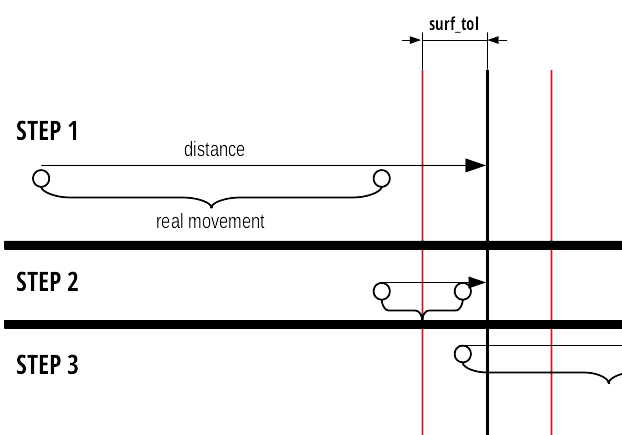
_images/UnderShot_SC.png — Self-correcting tendency for undershoots that lie outside surface tolerance.

Universe Polymorphism

Geometry of a nuclear reactor is structured. It is a collection of a large number of repetitions of simple arrangements such as fuel pins and fuel assemblies. Furthermore, these components are placed in a highly regular lattices. When reactor geometry is modelled in a MC code it is possible to use all this extra information about the structure to significantly accelerate geometry procedures. For example, in a Cartesian lattice with constant pitch it is possible to find a cell occupied by a particle with just few division and floor operations. Also the time required for the search is independent of the lattice size. Similar improvements can also be obtained for different arrangements like pin cells, fuel bundles or a pebble bed.

What is meant by universe polymorphism is that instead of creating few, very general representations of universes, a large number of highly specific universes is used instead. Each of them aims to address a particular geometrical arrangement encountered in reactor physics problems.

Components

This section is intended as a brief guide to the main components used in the SCONE geometry. Its purpose is to explain the logic and the intention behind why a particular component exists and what is its role.

Coord & Coord List

The purpose of the coords class in SCONE is to hold all the information related to a position of a particle in phase-space at a single level in the geometry. The coordList, as the name suggests, is a list of coords. It has a single entry for each level of the geometry. In addition it contains extra information about the material composition and the unique ID at the current position, which cannot be stored in coords since they are properties of a point in the domain, not of a point in a particular universe.

Furthermore coords:

contains information about rotations and translations of co-ordinate frame with respect to the previous level in the geometry

holds necessary information about position of a particle in a given universe: position (\(\bf{r}\)), direction (\(\bf{u}\)), local cell ID (localID), universe index (uniIdx) and position of the universe in graph representation of geometry structure (uniRootID)

(NOT YET IMPLEMENTED) holds cookies to allow universes to retain memory about a state. These are: position in a lattice (ijk) and a general cookie (mem) which is an arbitrary piece of memory stored as character. Such method is to allow universe to have some memory in a thread-safe fashion.

Furthermore coordList:

Contain current the number of levels occupied by the particle (nesting)

Hold material index (matIdx) and unique cell ID (uniqueID) for the current position of the particle

Hold a position of the particle in time

It is worth to note that the coordList can exist in three different states:

Uninitialised: All components of the coordList are unreliable and can take any values (e.g direction may not be normalised to one)

Above Geometry: Only position and direction at level 1 are reliable. matIdx and uniqueID are set to -ve values.

Inside Geometry: coords at all occupied levels (indicated by nesting) contain data that represents phase-space position at that level. matIdx and uniqueID are set to correct values.

Geometry Registry

Geometry registry is an object-like module (singleton) that manages the lifetime of different geometry and field definitions. A client code creates a geometry by providing the registry with a dictionary with its definition. Then it can be accessed from different places in the code via geomPtr function, which returns a pointer to initialised instance of the geometry. The same applies for a fields.

Geometry

Geometry is the primary interface for interaction with a geometry representation. It is intended to:

Perform movement of a particle. Note that what is actually moved in not the particle class, but the coordList.

Return pixel/voxel plots of the geometry

Return material/uniqueID at a given point in the geometry

Initialise (put) coordList in the geometry

Return axis-aligned bounding box (AABB) of the whole domain. If the box would stretch to infinity in some axis, width for that axis is assumed to be 0.

(NOT YET IMPLEMENTED) Return a pointer to a universe indicated by uniIdx

There are three types of movement in the geometry:

move: Standard movement of a particle. It moves up to a given distance or stops after crossing a boundary between regions with different materials or uniqueID. If the particle hits the domain boundary, boundary conditions are applied and the movement is stopped. It is also possible that a particle may become lost, as a result of errors in geometry handling. move can utilise the experimental distance caching if the cache is provided in the call.

move global: Movement with explicit tracking of the domain boundary. Particle moves up to a given distance “above” the geometry ignoring all changes in composition or unique ID. However, it will stop upon hitting the domain boundary (after BCs are applied).

teleport: Particle moves by a given distance without stooping. If it hits the domain boundary, boundary conditions are applied and the movement is continued

Surface

Surface exists to perform binary subdivision of the space into +ve and -ve halfspace. These halfspaces are used to define smaller volumes in the problem domain.

SCONE, does not limit the allowable surfaces to quadratic surfaces. More complicated shapes like boxes, truncated cylinders or parallelepiped are permitted. Each surface has an ID, which is a +ve integer and is used in geometry definitions in input file. Inside SCONE, a surface is identified by its index (surfIdx) different from its ID. Each surface:

determines a halfspace the particle is in (using surface tolerance)

calculates a distance along the flight to the next crossing between -ve and +ve halfspaces taking surface transparency into account

applies ordinary boundary conditions

applies co-ordinate transform boundary conditions

returns axis-aligned bounding box (AABB), that fully encompasses a surface. If the box would stretch to infinity in some axis, width for that axis is assumed to be 0.

Note

There is no check if the surface definitions are unique. Two surfaces that are exactly the same but have different ID can be defined (however there is no reason to do that and it should be avoided).
Each surface has its own value of surface tolerance. The SURF_TOL constant is more of a guideline really (surface tolerance of a surface aims to be as close to SURF_TOL as reasonably practicable [pun intended]. But for many surfaces (e.g. ellipses) exact equality would complicate code and hurt performance).

Cell

Cell exist as a separate objects only for convenience. They are intended to be used only by universes. Cell as a class represents a volume of space. It may or may not use any surfaces for its definition.

Universe

Universe represents a complete subdivision of the space into a disjoint regions (called local cells), each assigned with a local ID. Furthermore, it is a part of the geometry interface and client code may (if required) interact with universes directly (pointer to a universe can be obtained form geometry).

Each universe may be associated with an offset and/or rotation, which is applied to the coordinates upon entering the universe from a higher level.

Each local cell in a universe can also have an offset, which is a translation applied to co-ordinates before entering a lower level universe through the local cell. Thus, the position of a particle when it enters from a higher universe (0) to a lower universe (1) changes as follows:

\[\mathbf{r}_1 = \mathbf{r}_0 - \mathbf{R}_{uni} - \mathbf{R}_{cell}\]

Where \(\bf{R}_{uni}\) is the offset of universe 1 and \(\bf{R}_{cell}\) is the local cell offset from universe 0. Similarly, the direction and position of a particle can undergo a rotation, which is defined in terms of Euler angles (\(\phi, \theta, \psi\)) that follow so called x-convention:

\[\mathbf{A}= \left[ \begin{array}{ccc} \cos\psi \cos\phi - \cos\theta \sin\phi \sin\psi & \cos\psi \sin\phi + \cos\theta \cos\phi \sin\psi & \sin\psi \sin\theta \\ -\sin\psi \cos\phi - \cos\theta \sin\phi \cos\psi & -\sin\psi \sin\phi + \cos\theta \cos\phi \cos\psi & \cos\psi \sin\theta \\ \sin\theta \sin\phi & -\sin\theta \cos\phi & \cos\theta \\ \end{array} \right]\]

\[\mathbf{u}_1 = \mathbf{A} \mathbf{u}_0 \]

\[\mathbf{r}_{1r} = \mathbf{A} \mathbf{r}_1 \]

Note that the translation due to offset is performed before rotation. The x-convention for Euler angles is also called ZXZ because the 1st rotation (by \(\phi \in \left<0,2 \pi \right>\)) is performed over the Z-axis. The 2nd rotation (by \(\theta \in \left<0,\pi \right>\)) is around the rotated X-axis and the last rotation (by \(\psi \in \left<0,2 \pi \right>\)) is by the rotated Z-axis.

Note

Procedures for: distance, finding local cell, performing crossing are passed with universe with an intent inout, which means that they can modify a universe state. However, it can cause problems in parallel calculations. Thus, under normal circumstances these procedures should not change the state of a universe. If they do, it is responsibility of the programmer to ensure that these modifications would work in parallel calculations.
The procedure that calculates distance also returns a surface index, which is determined by the universe. It is used to identify a surface, which is the next boundary along the particle direction. Positive values of surfIdx indicate a surface that has been defined on surfaceShelf. Negative values indicate internal surfaces, that are defined only in the universe. The value of the surfIdx provided in distance calculation is returned as an input argument to the procedure that performs local cell crossings to potentially accelerate/simplify it.

Hole Universe

Hole universe is a special type of a universe that does not support distance calculations and local cell-to-cell crossings. It is named as a tribute to MONK Monte Carlo code. Like in MONK, hole universe represents a geometrical set-up which is unfeasible to model with surface tracking. However, it is still a subclass of universe so it must implement the distance & crossing procedures. Thus, if either of these procedures are called on a hole universe, execution is terminated with a fatal error.

Fields

Fields are special geometry objects that are meant to represents scalar and vector fields imposed over geometry. They take coordList as an input to have access to parameters such as matIdx or uniqueID, which might be useful when defining spatial variation of the field. For example, for an electric field, each material index may be associated with a different permittivity.

It is important to note that a field does not have to have physical interpretation. For example a field should be used to represent target weight distribution for weight windows variance reduction.

Note that for now both the vector and scalar are real. Fields might be extended to complex numbers in the future. Also fields have no implied representation. They can be just a single value in the entire space, they may be stored on a structured/unstructured mesh or some polynomial basis. The value of the field may also be completely independent of spatial co-ordinates and values might be assigned to regions by e.g. matIdx.

Geom Graph

As indicated in the previous section, the structure of the universe nesting may be represented by a directed acyclic graph. In SCONE this representation is decoupled from the description of the spatial subdivision (via universes). geomGraph is meant to hold the graph of the universe nesting. It:

accepts information about composition from universes during initialisation phase.

checks the validity of geometry structure

given a position of a universe in the graph (uniRootID) and local cell identifier (localID) it returns:

matIdx and uniqueID if the local cell contains material

uniIdx and new uniRootID if local cell contains a nested universe.

Geometry structure is considered valid if:

Special outside material is not present below the root universe

There is no recurrence in the universe structure (is acyclic)

Depth of the universe structure does not exceed the hardcoded limit (MAX_GEOM_NEST)

Currently geomGraph can be build as shrunk or extended. In extended configuration every instance of a material cell with a unique path in the graph is assigned with an its own uniqueID.

Note

The convention is that all matIdx are +ve. Thus, it is possible to use the sign bit to distinguish between material and universe fill stored in the same integer array.

Defining a geometry

It is probably best to discuss how to define a problem geometry in SCONE on an example. The sample problem consists of a single fuel rod with a square ‘core’. The dictionary with its definition is given below and the visualisation is shown in Figure 7

geometry {
  type geometryStd;
  boundary ( 1 1 2 2 0 0);
  graph { type shrunk; }

  surfaces {
    squareBound { id 1; type box; origin (0.0 0.0 0.0); halfwidth (5.0 5.0 5.0);}
    smallBound {id 2; type zSquareCylinder; origin (0.0 0.0 0.0); halfwidth (0.3 0.3 0.0);}
   }

  cells {
    inner {id 1; type simpleCell; surfaces (-2); filltype mat; material core;}
    outer {id 3; type simpleCell; surfaces (2); filltype mat; material cover;}
  }

  universes {
    root { id 1; type rootUniverse; border 1; fill u<10>;}

    pin31 { id 10;
            type pinUniverse;
            origin (1.0 0.0 0.0); rotation (0.0 30.0 0.0);
            radii (0.900 0.0 ); fills (u<11> water);
          }

    cellUni { id 11;
              type cellUniverse;
              cells (1 3);
            }
  }
}

The definition of the geometry is specified in a sub-dictionary (in the main input file) called geometry, which must contain four additional sub-dictionaries: graph, surfaces, cells and universes. In addition, keywords type and boundary must be provided. The former specifies the type of the geometry to be build (only geometryStd is available at the moment), the latter contains a list of integers to specify boundary conditions (0-Vacuum, 1-Reflective, 2-Periodic). The association between the integers and faces of a boundary surface depends on the surface type. Thus, check the documentation comment of a particular surface type for details.

_images/x_cut.png — Visualisation of the geometry. Plane is normal to x axis through point \((1,0,0)\)

Meaning of each sub-dictionary is obvious. For extra details please refer to documentation comments of geomGraph, surfaceShelf, cellShelf and universeShelf types. Please remember that in Sample dictionary input section hashes (#...#) mark optional entries. It is also worth to note that when a material filling needs to be specified in a universe definitions, a nested universe can be placed there instead with the u<uni_id> syntax. The only exceptions are fillings of cells, where the filling type needs to be explicitly specified. The question that probably comes to your mind right now is “what will happen if I name a material e.g. u<223>?”. The answer is that it will be interpreted as universe with id 233, without any warning.

Unfortunately at the moment reference to different surfaces, universes and cells is made only by id, which must be a positive integer. Sadly, it significantly reduces the readability of an input file. The official excuse why it is the case is the usual strings are messy in Fortran. We will try to do better in the future…

SCONE has a major restriction on a root universe (1st top level universe) in the geometry definition. It has to be of type rootUniverse, which is composed of a single surface that separates the entire space into inside and outside region. In the example above this special universe is included in universes sub-dictionary under keyword root, which is a default. Different keyword may be used by providing the universe id by root entry in the geometry dictionary (see csg class for details ).

The reason for this quirky requirement is the combination of the use of body surfaces (e.g. box) and support for both the co-ordinate transform and explicit boundary conditions. The co-ordinate transform treatment forces a requirement for the domain boundary to be composed of a single computational surface only (e.g. box). This, on the other hand, creates a problem in a case of a partial surface overlap with the boundary surface on the root level (e.g. where two boxes share a part of a face). Under this conditions it is possible for a particle to hit the non-boundary surface and after the cell crossing end up outside the domain. Since it does so without hitting the boundary surface explicitly, no boundary condition is applied and the particle always leaks. The easiest way to avoid this problem is to have a root universe defined with a single (boundary) surface.

Further examples of working geometries are available in the InputFiles directory in the code repository. Also note that the maximum depth of the geometry in SCONE is hard-coded. If you want to create geometry deeper than allowed, change HARDCODED_MAX_NEST in UniversalVariables.f90 and recompile.

Note

Refer to documentation comments for syntax and details: Do it since the details of the syntax required do define different surfaces, cells or universes is provided only in the documentation comments of their respective classes (in Sample Input Dictionary section). Information there will always be up-to-date.

References

[Salvat]

F. Salvat, “PENELOPE-2014: A Code System for Monte Carlo Simulation of Electron and Photon Transport”, NEA, NEA/NSC/DOC(2015)3, 2015.

[Briesmeister]

1. Briesmeister, “MCNP - A General Monte Carlo N-Particle Transport Code”, LANL, LA-13709-M, 2000.